Computing Inequality Metrics

import numpy as np
import matplotlib.pyplot as plt

from salamanca import ineq

% matplotlib inline

Measures of Inequality

The most common measure of inequality is the Gini coefficient. A less common measure is the Theil coefficient, but it has nice mathematical properties that allow it be decomposed and recomposed based on subpopulations.

There is a theoretical and statistical relationship between Theil and Gini:

\[t(g) = \sqrt{2} \Phi^{-1} \left( \frac{1+g}{2}\right)\]

Where \(\Phi\) is cumulative distribution function (CDF) of the standard normal distribution.

We can compute values as follows:

gini = 0.5
theil = ineq.gini_to_theil(gini)
theil

0.45493642311957266

Empirical work has been done which shows that Theil values from household data surveys do not match exactly with Theils as computed from theoretical distributions. The difference in values are approximately 10%.

theil_emp = ineq.gini_to_theil(gini, empirical=True)
theil_emp

0.41796418400726093

rel_diff = (theil - theil_emp) / theil
rel_diff

0.081269024051288552

Distributions

Income is most commonly modeled as lognormal distribution (though there is gaining momentum amongst economists to use a duel-tailed Paretto distribution).

dist = ineq.LogNormal(inc=1000, gini=0.4)
x = np.linspace(dist.ppf(0.1), dist.ppf(0.9), 100)
y = dist.pdf(x)
plt.plot(x, y)
plt.xlabel('Income'); plt.ylabel('Population (relative)')

<matplotlib.text.Text at 0x7f5ea1880b90>

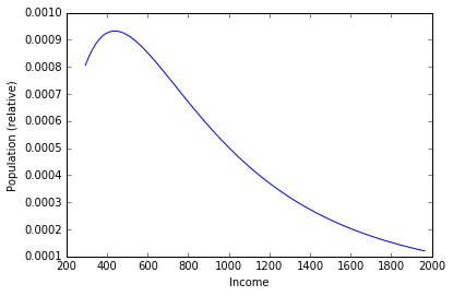
By default, salamanca assumes you wish for the distribution’s income to be defined by its mean value.

dist.mean()

1000.0000000000001

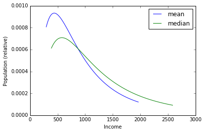
However, this can be changed to assume that the income is a median income.

for ismean in [True, False]:
    x = np.linspace(dist.ppf(0.1, mean=ismean), dist.ppf(0.9, mean=ismean), 100)
    y = dist.pdf(x, mean=ismean)
    label = 'mean' if ismean else 'median'
    plt.plot(x, y, label=label)
plt.xlabel('Income'); plt.ylabel('Population (relative)'); plt.legend(loc='best')

<matplotlib.legend.Legend at 0x7f5e9ff5cf90>

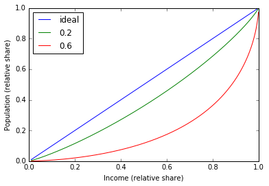
Lorenz Curves

Lorenz curves are a common way to view income distributions from an inequality lens.

x = np.linspace(0.01, 0.999, 1000)
plt.plot(x, x, label='ideal')
for gini in [0.2, 0.6]:
    y = dist.lorenz(x, gini=gini)
    plt.plot(x, y, label=str(gini))
plt.xlabel('Income (relative share)'); plt.ylabel('Population (relative share)'); plt.legend(loc='best')

<matplotlib.legend.Legend at 0x7f5e9ddd4ed0>

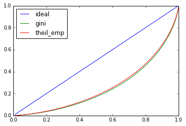
We can again see the effect of applying the empirical Theil relationship on the Lorenz curves.

gini = 0.5
theil = ineq.gini_to_theil(gini, empirical=True)
plt.plot(x, x, label='ideal')
plt.plot(x, dist.lorenz(x, gini=gini), label='gini')
plt.plot(x, dist.lorenz(x, theil=theil, gini=None), label='theil_emp')
plt.legend(loc='best')

<matplotlib.legend.Legend at 0x7f5e9dd30790>

Populations below Income Thresholds

A common application of inequality calculations is to determine the fractions of populations in various income quantiles. A convenience function is provided to make this straightforward.

dist = ineq.LogNormal(inc=1000, gini=0.4)
dist.below_threshold(500) # ~ 30% makes less than 500

0.28643175826024936

dist.below_threshold(1500) # ~ 80% makes less than 1500

0.82057020130849057